Learning and Compression

Learning and compression have inextricable connections. As David MacKay said, machine learning and information theory are the two sides of the same coin. The beautiful part of the connections, at least to me, is that those connections can be mathematically derived. I’d like to introduce the connections for people who are also fascinated by the connections between these two. For each part, I will first introduce the intuition, and then the formal derivation so for folks who are only interested in high-level ideas can (hopefully) get some inspirations too.

When (Unsupervised) Learning is Compression

Intuition

Shannon’s source coding theorem was originally developed to solve communication problems. The purpose of communication is to make sure the message from the sender is delivered to the receiver. Pretty straightforward right?

Now I want to send a message to you by showing a picture:

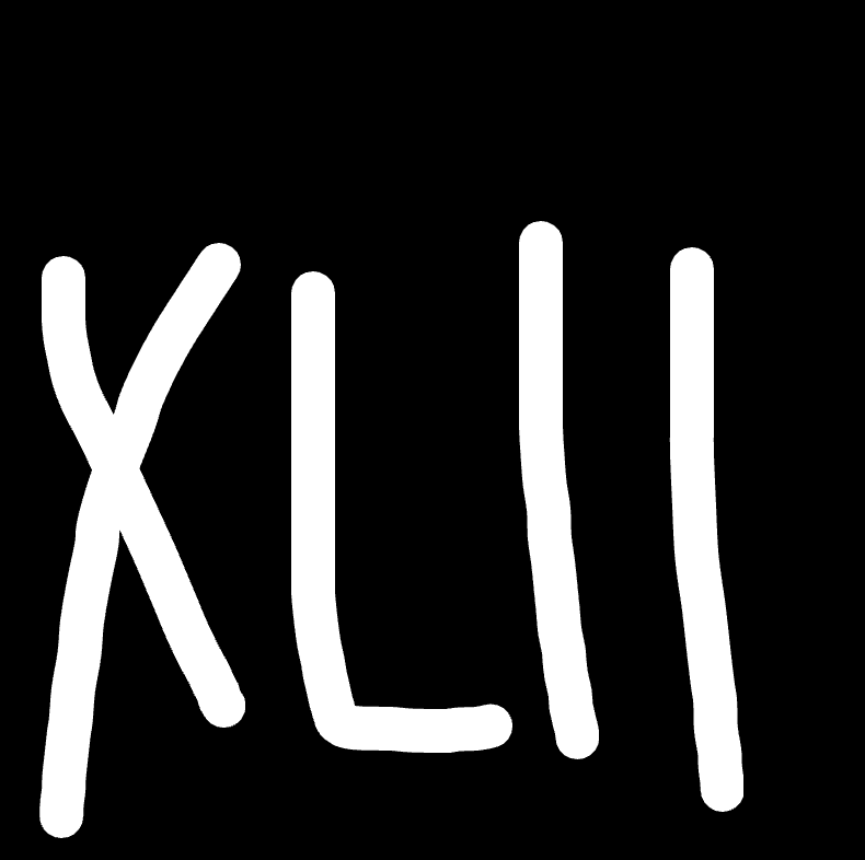
(Assuming) You look puzzled and are not sure what message I’d like to send. So I send more pictures:

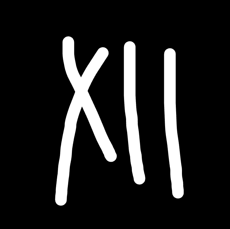
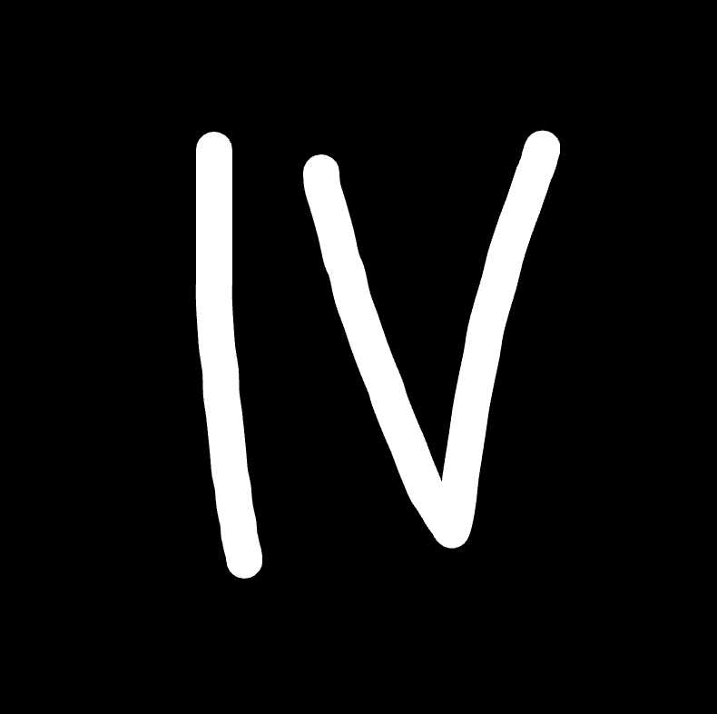
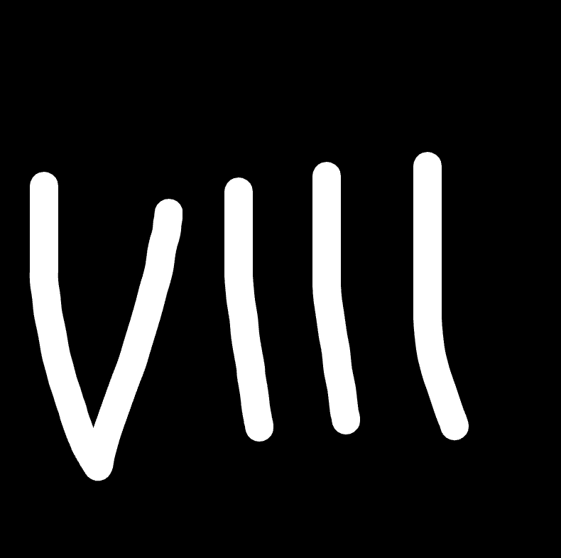
(Still assuming) You now have a clue that the image I sent earlier might be about roman number.

What just happened? Why sending more images without telling you what is the first image can help you get more information about the first image?

Two important things are happening if you do think the first image is about roman number:

1. You assume the first image and the subsequent images come from the same distribution.
2. You are trying to capture regularity/recognize patterns through those images.

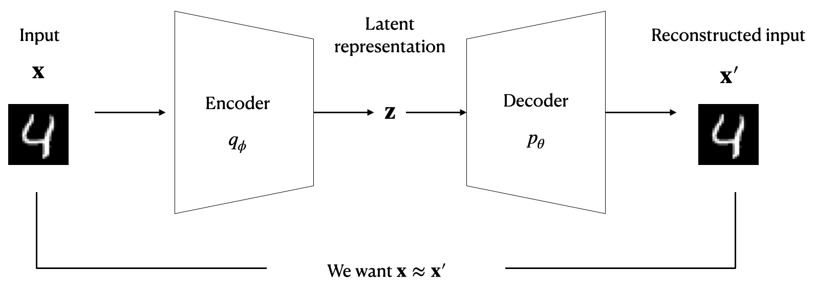
During the process of trying to figure out what’s the pattern underlying all those images, without any labels, you are doing unsupervised learning. More specifically, the figure below describes what we just did. Encoder here can be understood as me (specifically my thought process of converting the message into the image plus my handwriting process 🤗).

We can understand the unsupervised learning from below two perspectives, loosely speaking:

1. From generative models perspective: The procedure of unsupervised learning is to learn to capture regularity. The measurement of how well the regularity is captured is often reflected by how short the estimated compressed length can be. Therefore, we can directly use the estimated compressed length as our objective function.
2. From message length perspective: As a decoder, you were trying to recover the message I’d like to send. You learn about the correctness by checking with me. Corresponding to unsupervised training on images or texts, we do not have any labels available. So we use the original input source as our ground truth, and compare the output by decoder with the ground truth. The learning procedure is actually learning the data distribution that the input images/texts come from and try to re-generate/recover them as close to the input as possible.

(“The answer is 42.”)

Derivation

The above two perspectives are mathematically equivalent with certain assumptions. To be specific, generative models with explicit density estimation can be used as compressors anyways. It’s just we often need certain types of coding schemes to convert probability distribution to binary codes. However, when the objective function of generative models is equivalent to minimizing code length, we can use the value of objective function directly as estimated compressed length. Those generative models include but are not limited to: variational autoencoders, autoregressive models, and flow models. I will walk you through the derivation of the equivalence of commonly used ones.

VAE

Following the example, let’s first dive into variational autoencoder (VAE), which has similar encoder-decoder architecture as the example above.

Remember from the perspective of generative models, we were trying to learn the data distribution so that we can generate the input message. Then let’s just look into the data distribution:

The problem is that the above equation is intractable. So we introduce another more “controllable” distribution q_\phi(\mathbf{z}\vert\mathbf{x}) to approximate p(\mathbf{z}\vert\mathbf{x}), which enables us to derive a lowerbound (\phi, \theta here indicates the distribution is modeled by neural networks with learnable parameters):

The RHS is the typical loss function of VAE, which is called evidence lowerbound (ELBO).

Now let’s start from the message length perspective.

Following the tradition, let’s assume we have a sender named Alice and a receiver named Bob. This part of derivation relies on the prior knowledge of “bits-back” argument. To put it simply, we assume Alice has some extra bits that she’d like to send alongside with the original message. This extra bits can be understood as some kind of seed for Alice to draw sample from. It’s also assumed that both Alice and Bob have access to $p(\mathbf{z})$, $p_{\theta }(\mathbf{x}|\mathbf{z})$, $q_{\varphi }(\mathbf{z}|\mathbf{x})$, where $p(\mathbf{z})$ is the prior distribution, $p_{\theta }(\mathbf{x}|\mathbf{z})$ is a generative model and $q_{\varphi }(\mathbf{z}|\mathbf{x})$ is the inference model.

Then the procedure of Alice sending a message can be summarized as the figure below: Alice first decodes the extra information according to $q_{\varphi }(\mathbf{z}|\mathbf{x})$, $\mathbf{z}$ is further used to encode $\mathbf{x}$ with $p(\mathbf{x}|\mathbf{z})$ and $\mathbf{z}$ is encoded using $p_{\theta }(\mathbf{z})$.

The total length of final bistream is therefore:

Now we can see that optimizing latent variable models (learning) is equivalent to minimizing the code length (compression) through bits-back coding using the model !

GPT (and other Autoregressive models)

The equivalence between Autoregressive models’s loss function and minimizing message length is pretty obvious.

Starting from probabilistic modeling (generative model) perspective, we still want to model the probability distribution \log p(\mathbf{x}). Now we are modeling autoregressive models, which means:

Unlike VAE, this log likelihood can be calculated empirically, so we use this function as our objective function directly in autoregressive models.

From the message length perspective, Shannon’s entropy told us that the minimum code length we can achieve is H(\mathbf{x})\triangleq \mathbb{E}[-\log p_{\text{data}}(\mathbf{x})], where p_\text{data} represents the ground truth of the data distribution. While p_\text{data}(\mathbf{x}) is unknown to us, we can use p(\mathbf{x}) to approximate, by learning from next-token prediction through samples from the distribution. This is demonstrated in details in Ref[9] and Ref[10].

Summary

This part can be summarized into two main points:

1. Optimizing certain generative models = Minimizing code length
2. The value of loss function of VAE and GPT can be used as estimated code length.

When Compression Helps (Supervised) Learning

Intuition

Let’s look at two images below

Now cover these two images, can you answer: which image has the orange strip on the left, the top one or the bottom one?

Intuitively, we feel these two images are “similar” in some sense that are hard to be differentiated easily.

Obviously, the euclidean distance is large. Then how can this similarity be measured?

To get some inspirations, let’s take a look at another two images

The common part between flag-like pairs and Spock pairs is that they both can be converted from one to another easily. To convert colored-Spock to greyscaled-Spock, we can use, for example, python code${}^{[0]}$:

Similarly, we can use python code to convert the flag-like images:

The common part between the two programs is that they are both short. Naively, we can say the similarity that reflects our intuition can be captured by “the minimum length of the program that converts one object to another”. The minimum here asks for the best version of the converting program.

How does “the minimum length of the program that converts one object to another” have anything to do with compression?

Intuitively, a compressor like gzip can be viewed as a “program”, the inner algorithm decides how well the compressor as a program can compress. Regardless of how well the compressor can do, the primary purpose of a lossless compressor is to use as least bits as possible by capturing the regularity and reducing redundancy. The conversion can be viewed as “compress input A given input B”.

Once we have a similarity/distance metric, we can measure the distance between test samples and training samples and use labels of nearest training samples to inform the prediction of test samples.

We will now convert this intuition into the derivation of our distance metric and method step by step.

Derivation

“The minimum length of the program that converts one object to another” can be formalized as information distance, defined as:

where K(x\vert y) represents conditional Kolmogorov complexity, meaning the minimum length of the (binary) program that produces x given y, K(xy) means the length of the shortest binary program computing x and y (without separator encoded).

Kolmogorov complexity

To understand K(x\vert y), let’s first look at the vanilla version, K(x). K(x) is the length of the shortest binary program that can produce x on a universal computer U:

The development of Kolmogorov complexity originates from the need to define “randomness”. The intuition is quite simple - random sequences are sequences that cannot be compressed.

Take an example below:

Before figuring out the regularity inside s, we will use 147 (\log_2 149162536496481100121144169196225256289324361) bits to represent s. But if we observe carefully, we can find s can be represented by:

Converting for-loop into a binary program is a constant, so the length of the above program is just O(\log_2 20)+O(1)^{[2]}. It is like when we are learning geometric series, we just need to know the initial value a, the ratio r and we know all the sequences - the description length is extremely short as the regularity can be “described” in a very simple way.

In other words, Kolmogorov complexity K(x) can be viewed as the length of x after being maximally compressed.

Similarly, K(x\vert y) can be understood as the length of x after being maximally compressed given the information of y.

Now the problem is, how can we possibly find the shortest program? Sadly, we can’t. Kolmogorov complexity is incomputable^{[3]}. But remember, K(x) can be viewed as the length of x after being maximally compressed! That means, we can use a compressor to approximate K(x).

Information Distance

What about E(x,y) then? How to approximate that? I will show how to derive from information distance E(x,y) to a computable distance metric.

First, let’s start with a normalized version of information distance (NID), so that the distance value ranges from 0 to 1:

Now, let’s assume K(y)\geq K(x), we then have:

where I(x:y)=K(y)-K(y\vert x) means the mutual algorithmic information. \frac{I(x:y)}{K(y)} means how many bits of shared information, per bit of information contained in the most informative sequence.

Loosely, NID can be understood as: how many “percentage” of bits we still need to output y if we know x.

A simple diagram below may illustrate the relationship between K(x\vert y), I(x:y), and K(y\vert x).

To derive a computable version of the metric, we need to figure out one more thing in addition to approximating K(x) - how to approximate the conditional Kolmogorov complexity K(x\vert y). Why? Because for traditional compressors like gzip, it’s not obvious how to compress x given y. (things will be different for neural compressors, and we will cover it later.)

Therefore, we use the second equation of information distance $E(x,y)=K(xy)-min\{K(x),K(y)\}$ in NID. As a result, the final NID is represented with only K(xy), K(x), K(y) without any conditional Kolmogorov complexity. Replacing all the K(x) with C(x), which is denoted as the compressed length given by a compressor, we have Normalized Compression Distance (NCD):

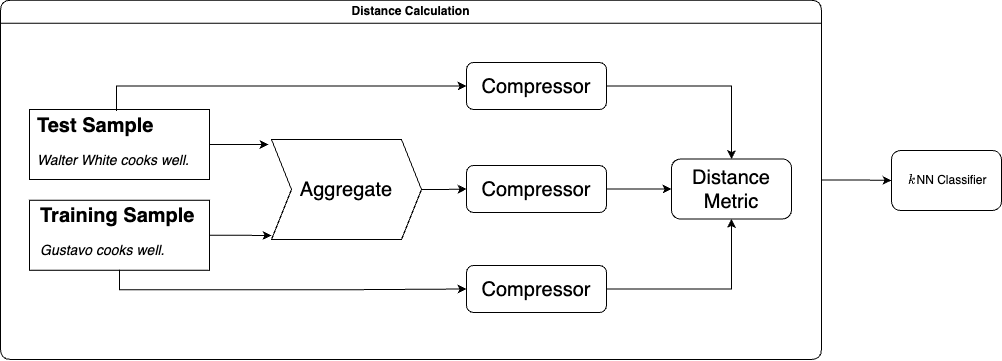
Once we have a way to measure the distance/similarity between two samples, we can use metric-based methods like k-Nearest-Neighbor (kNN) classifier for supervised learning, the pseudo code is like follows:

Summary

Overall, the procedure of “how can compressor help supervised learning” can be summarized in the plot below:

When the above two combined

Now we’ve known

1. Unsupervised learning can be viewed as compression.
2. Compression can help supervised learning.

What does it indicate?

The approximation of information distance relies on the approximation of Kolmogorov complexity, and as the unsupervised learning optimizes towards the minimum code length, Kolmogorov complexity can be better approximated with the help of unsupervised learning!

In this way, we can capture the data distribution belonging to each dataset and we can utilize the distribution we captured to improve downstream supervised tasks with ease!

Neural Compressor based Classification

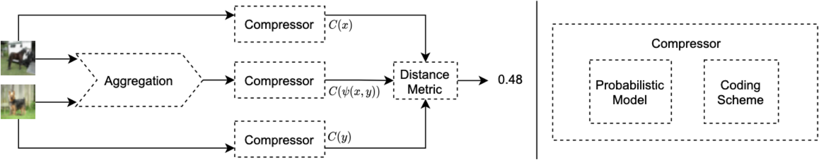
Based on the above, we can decompose NPC framework into three main components as shown in the figure: a compressor, a distance metric, and an aggregation method. The compressor consists of a probabilistic model and a coding scheme. And we then use deep generative models with explicit density estimation (e.g., GPT) as probabilistic model.

VAE as a Compressor for Classification

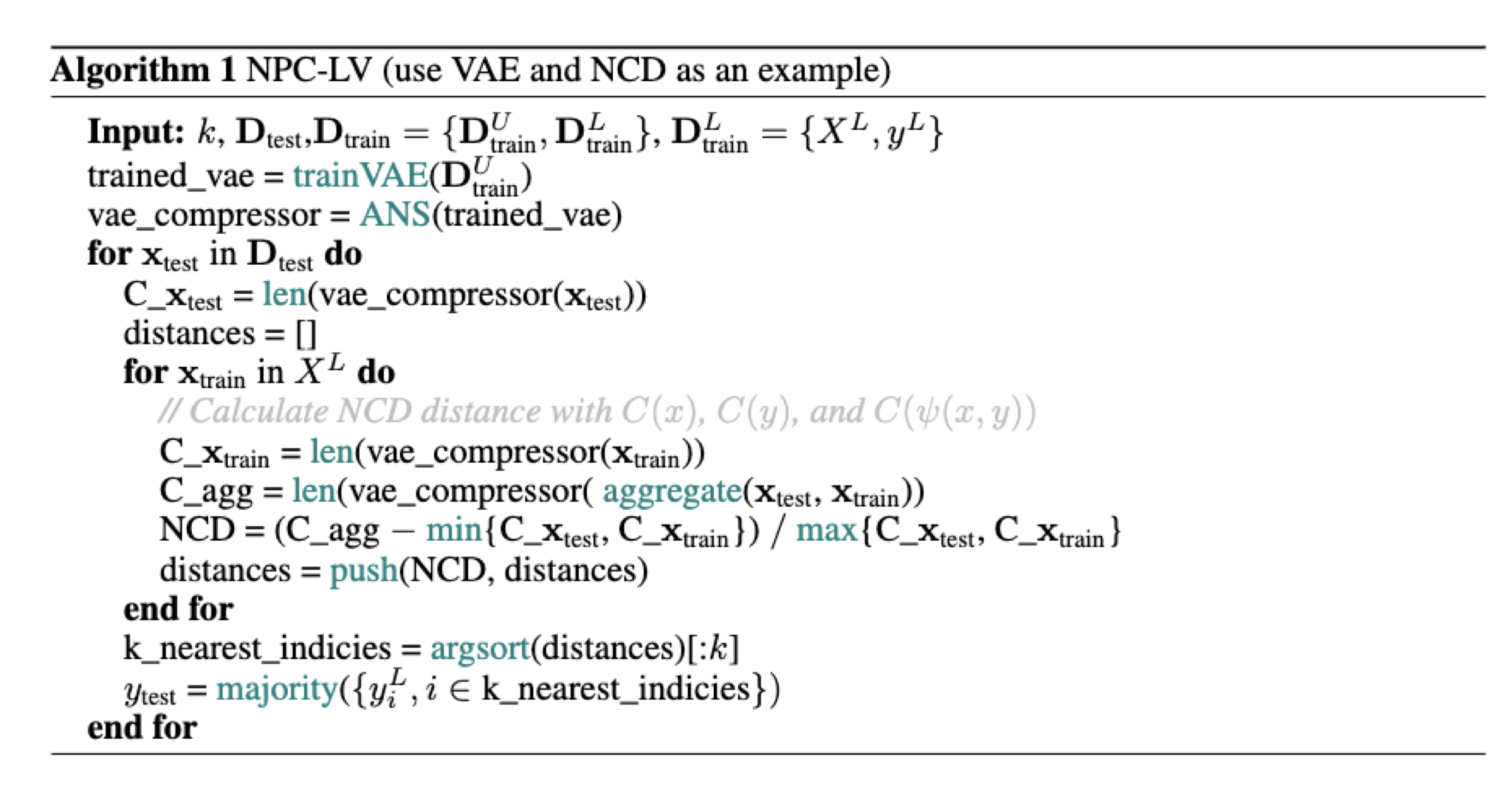
Let’s first take VAE-based compressor with NCD as a concrete example. The steps of combining unsupervised learning and supervised learning are as follows:

1. We first train a VAE on the unlabeled training set
2. Optional: Apply ANS with discretization on the trained VAE to get a compressor
3. We then Calculate the distance matrix between pairs with the compressor and NCD
4. Finally we Run kNN classifier with the distance matrix

The second step is optional as we can use nELBO as estimated compressed length directly without any discretization or coding scheme.

GPT as a Compressor for Classification

It’s similar to the traditional compressor except that we replace “Compressor” with “GPT”.

How does this intuition translate into code?

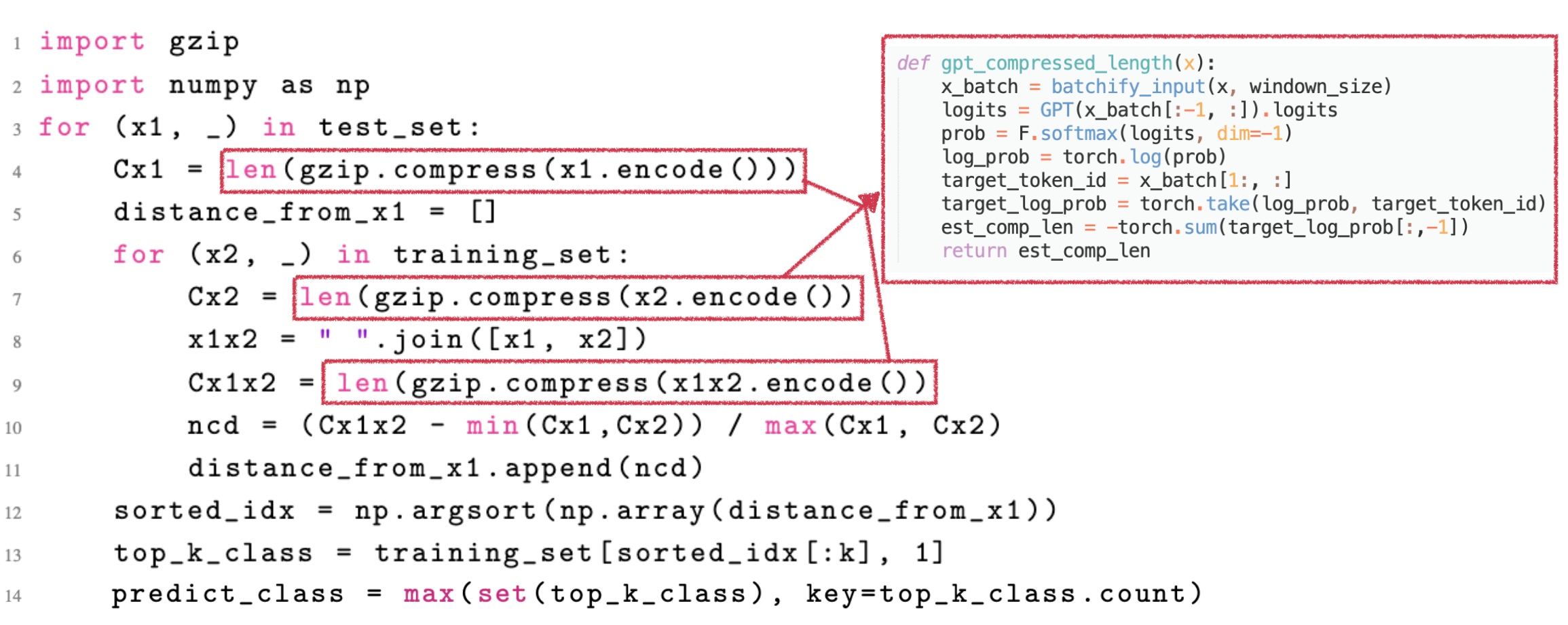
Pretty simple, something like the figure above shows. The only difference is the logic of computing the compressed length. So instead of using gzip to compress text, we are using GPT to estimate the compressed length of the text, which is just the sum of the log probability of the target tokens.

For those who are interested in the experimental results of using VAE and GPT as compressors for classification, you can check Ref[7] and Ref[9] respectively.

Summary

We see that it’s pretty straightforward to just use either nELBO or log probability directly for classification. So you can either use models that pretrained on huge datasets like GPT or use a smaller models pretrained on a local smaller unlabeled dataset like the example of VAE.

Footnote

[0] I also want to mention one irrelevant detail here: averaging RGB channels is just an approximation to greyscale. As our eyes actually perceive the luminance of red, green and blue differently, if you want to calculate the real greyscale image, those three channels will have different weights, but still it’s linear combination of three colours.

[1] For people who are extremely curious, you may wonder why there is \max for the information distance. A simpler version of the answer is that \max makes sure the information distance satisfies the symmetry axiom, which is the requirement if we want to define something as metric. Then why it’s \max instead of \min? Assume K(y\vert x) > K(x\vert y), using \min can only guarantee the one-way conversion. Please also note that the second equation works up to $O(\log K(x,y))$.

[2] The exact length will differ with different programming languages. But invariance theorem states that the difference caused by programming languages is a negligible constant.

[3] The proof is classic - through contradiction and self-reference. https://en.wikipedia.org/wiki/Kolmogorov_complexity

Reference

[0] David JC MacKay. Information theory, inference and learning algorithms. Cambridge University Press, 2003.

[1] Brendan J Frey and Geoffrey E. Hinton. Efficient stochastic source coding and an application to a bayesian network source model. The Computer Journal, 40(2):157–165, 1997.

[2] Jarek Duda. Asymmetric numeral systems. arXiv preprint arXiv:0902.0271, 2009.

[3] Charles H Bennett, Péter Gács, Ming Li, Paul MB Vitányi, and Wojciech H Zurek. Information distance. IEEE Transactions on Information Theory, 44(4):1407–1423, 1998.

[4] Ming Li, Xin Chen, Xin Li, Bin Ma, and Paul MB Vitányi. The similarity metric. IEEE
transactions on Information Theory, 50(12):3250–3264, 2004.

[5] James Townsend, Thomas Bird, and David Barber. Practical lossless compression with latent variables using bits back coding. In International Conference on Learning Representations (ICLR), 2019.

[6] Andrei N Kolmogorov. On tables of random numbers. pages 369–376, 1963.

[7] Zhiying Jiang, Yiqin Dai, Ji Xin, Ming Li, and Jimmy Lin. “Few-shot non-parametric learning with deep latent variable model.” Advances in Neural Information Processing Systems 36 (2022).

[8] Zhiying Jiang, Matthew Yang, Mikhail Tsirlin, Raphael Tang, Yiqin Dai, and Jimmy Lin. ““Low-Resource” Text Classification: A Parameter-Free Classification Method with Compressors.” In Findings of the Association for Computational Linguistics: ACL 2023.

[9] Huang, Cynthia, Yuqing Xie, Zhiying Jiang*, Jimmy Lin, and Ming Li. “Approximating Human-Like Few-shot Learning with GPT-based Compression.” arXiv preprint arXiv:2308.06942 (2023).

[10] Delétang, Grégoire, Anian Ruoss, Paul-Ambroise Duquenne, Elliot Catt, Tim Genewein, Christopher Mattern, Jordi Grau-Moya et al. “Language modeling is compression.” arXiv preprint arXiv:2309.10668 (2023).