gzip+kNN

Finally got a chance (after 5 months!) to write something less formal and talk about my personal thoughts on the gzip paper$^{[1]}$.

I realized our paper has received some attention, with most reactions on two extreme sides. I personally think our paper is similar to most papers in that it has both inspirational part and limitations. So I really appreciate people like Sebastian and Abhinav who introduced the idea in a responsible way.

tl;dr

I think gzip+knn is overhyped, but the framework and theory behind is not.
The original code didn’t have a bug of calculating top $k$ accuracy. It calculates the maximum accuracy when tied. It is documented in the paper Appendix C in the first place$^{[2]}$.
Some people mentioned using “maximum” as tied strategy is an unfair comparison, so we add result using “random” strategy when tied. Only look at “random” result, the conclusion is that:
(1). In the few-shot settings, gzip(rand) outperforms all methods on Kinyarwanda, Kirundi, Filipino, and SogouNews but is worse than mBERT on Swahili, on which mBERT has been pretained.
(2). In the full dataset setting, gzip(rand) is only highest on SogouNews, is competitive on Kinyarwanda and Swahili, and is bad on Kirundi and updated DengueFilipino.
Considering the NFL theorem, gzip is leaning towards the “universal” side.
For practitioners, when to use gzip? (1) When you have no prior knowledge about the datasets and only have few labeled data available (few-shot scenario); or (2) When the datasets are very compressible (in both full and few-shot settings).

In this blog, I will briefly recap the main idea, then discuss about tie-breaking strategy and added results, also go into practical guide and limitations, and my personal thoughts about its future work.

Main Idea

Intuition

Compressors are good at capturing regularity.
Objects from the same category share more regularity than those from different categories.

This might be clear with text examples:

$x_1$ = “US’s Stark Industries has developed a 12-gram flying microrobot.”
$x_2$ = “The latest tiny flying robot has been unveiled in US.”
$x_3$ = “Quicksilver won the gold medal in the 400 individual medley.”

If we only compress $x_2$, the compressed length is $72$ bytes, and let’s denote it by $C({x_2})$. Similarly, only compressing $x_3$ gives us $C({x_3})=72$, too (this is a coincidence…).

Now what about $C({x_1}{x_2})$ and $C(x_1x_3)$, are they the same too?

Using len(gzip.compress(x.encode('utf-8'))) we get $C({x_1}{x_2})=122$ and $C({x_1}{x_3})=130$.

Why is $C({x_1}{x_2}) < C({x_1}{x_3})$?

Because the information in $x_1$ helps the compression of $x_2$ more than it helps $x_3$. In other words, $x_1$ and $x_2$ share more common patterns. It’s also pretty obvious that $x_1$ and $x_2$ belong to $\texttt{techonology}$ category, while $x_3$ belongs to $\texttt{sports}$ category.

But you may also notice that only using the compressed length of concatenation like $C(x_1x_2)$ to compare around is not enough - what if $x_2$ is super long while $x_3$ is super short? We need to have a way to measure the averaged value of “how much information we still need in order to compress a new string”.

This is the motivation for a formally defined metric Information Distance$^{[3]}$ and the subsequent normalized version: Normalized Information Distance. To put it simply, Information Distance between $x_1$ and $x_2$ means the length of the shortest program that can convert from $x_1$ to $x_2$ on a universal computer.

For example, for two images below,

one of the programs that can convert from one to another can be:

import numpy as np img2 = np.fliplr(img1)

Information Distance

Information Distance is a desirable distance metric as among all “reasonable”$^{[5]}$ distance metrics, it’s the minimum one$^{[6]}$. The problem is that Information Distance is not computable. Looking at the above python program, you may have already had an intuition about why it’s not computable - it’s hard to know whether the program you wrote is the shortest one$^{[4]}$. Instead, you can just approximate the shortest one.

To have a computable version of information distance, Normalized Compression Distance (NCD) is defined$^{[6]}$, which is the distance metric used in all the experiments. Basically, NCD uses compressors to approximate the shortest program that can convert one object to another, and it normalizes this value so that the length of the original object won’t matter a lot. If you are interested in how to derive NCD, I wrote another blog to introduce the derivation in detail.

With the help of NCD, we can calculate the distance between any two objects. So when we have a test data point $x_{test}$, we can use NCD to calculate the distance between $x_{test}$ and other training points. We then predict $x_{test}$’s label by the majority vote of training points’ labels (the high-level summary about $k$-nearest-neighbor classifier).

Concerns Regarding to Accuracy Calculation

There have been a lot of discussions$^{[7]}$ surrounding the reported accuracy - whether it’s top-$k$ accuracy, whether it’s a fair comparison, etc. I’d like to clarify misconceptions about top-$k$ accuracy and share added results as well as comments on this issue.

Choice of $k$

Traditionally in $k$NN, the rule of thumb to pick $k$ is to use $\sqrt{n}$, where $n$ is the number of training samples$^{[6]}$. In our experiments, we have both full-data setting and few-shot setting, where only very limited number of labeled data are given. In order to use one $k$ for all experiments and fit the 5-shot setting, we use $\sqrt{5}\approx 2$. But setting $k$ to an even number is not a great choice and we will see the reason in a minute.

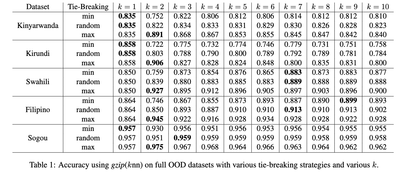
Tie-Breaking Strategy

When we use “majority vote”, there are chances we have different classes with same number of votes. For example, when $k=5$, we have 2 votes for class $\texttt{sports}$, 2 votes for class $\texttt{politics}$ and 1 vote for class $\texttt{tech}$. We then have a “tie” situation for $\texttt{sports}$ and $\texttt{politics}$. This “tie” situation happens more when we have an even number. We need some strategies to break the tie and choose either $\texttt{sports}$ or $\texttt{politics}$.

The simplest strategy is random - just pick tied classes randomly (this can be set via rand=True flag in the original codebase). As you can imagine, the accuracy with random will be unstable, depending on how lucky we are. This becomes trickier under few-shot settings as we will have more randomness with different training samples being picked.

What should we do if we’d like to have a more stable accuracy? Increase the trials of experiments. Currently we have repeated $5$ times under each few-shot setting and have run a total number of $85$ few-shot experiments. Suppose we use random strategy and repeat each experiment for $5$ times, we need to run $425$ experiments to have a more stable result!

So we report the result with a more deterministic strategy - maximum, which assumes we are super lucky and always guess the label correctly when tie. In other words, this is the upperbound of the accuracy we can get with gzip+$k$NN.

We also use maximum strategy for other methods utilizing $k$NN, including word2vec and sentenceBERT. This choice is documented in Appendix C of the original paper.

Why it’s not top-$k$ accuracy

Below is the code snippet that deals with accuracy calculation, and it is thought to be a bug of calculating top-$k$ accuracy:

for pair in sorted_pred_lab: if pair[1] < most_count: break if not rand: if pair[0] == label[i]: if_right = 1 most_label = pair[0] else: most_voted_labels.append(pair[0])

I will explain why the code doesn’t calculate top-$k$ accuracy and why it’s thought to be.

What is the definition of top-$k$ accuracy exactly? Below is the definition copied from scikit-learn:

It computes the number of times where the correct label is among the top $k$ labels (ranked by predicted scores) predicted. $^{[8]}$ [Def.1]

Now recall that discriminative models like BERT will output a list of predicted classes with scores before picking the most possible one. Take trinary classification as an example, suppose we have only three classes - tech, sports, and politics, we will have probability predicted for each model like below:

BERT:

tech: 0.73
sports: 0.24
politics: 0.03

While for models like $k$NN, take the same trinary classification as an example, suppose we set $k=3$, the step before picking the most possible one is to have $k$ labels belonging to the nearest instances, so we will have something like below:

kNN:

tech
tech
sports

Suppose the ground truth is sports and we are calculating top3 accuracy. For BERT, we will score every time but for $k$NN, we will not. In fact, BERT will have 100% accuracy for top3 accuracy while $k$NN will have the accuracy way lower.

The difference of accuracy between discriminative models like BERT and $k$NN is that - We are implicitly using different definitions of top-$k$ accuracy for $k$NN. The top-$k$ accuracy for $k$NN in the above example actually means:

The percentage of nearest $k$ labels that contain the ground truth. [Def.2]

[Def.2] is clearly different from [Def.1], which is the definition of top-$k$ accuracy, and accuracy calculated using [Def.1] is way higher than accuracy calculated using [Def.2].

But why it’s thought to be calculating top-$k$ accuracy? Because if we incorrectly use [Def.2] to calculate top2 accuracy for $k$NN, we will get the same numerical value as using maximum strategy when tied if $k=2$.

In summary, when $k\neq 2$, the code snippet doesn’t calculate top-$k$ accuracy either logically or numerically; when $k=2$, the code snippet doesn’t calculate top-$k$ accuracy logically but generates the same numerical value under [Def.2], which is actually not the definition of top-$k$ accuracy.

Unfair Comparison

Although the reported accuracy is not top-$k$, only comparing the upperbound of gzip+$k$NN to other methods is still an unfair comparison. I do agree that reporting maximum only is not enough and including random and minimum can provide a more wholistic point of view. So here is the updated table that I posted during the discussion:

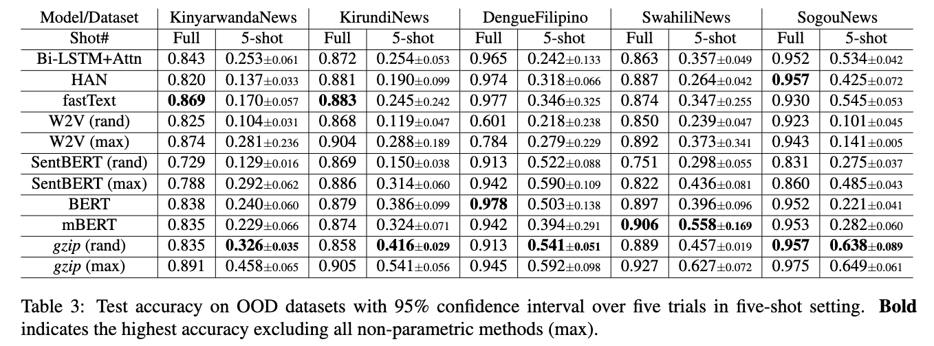
Results for W2V and SentBERT under random are also included for comparison. So if we only compare the result with random, we can see that under 5-shot settings, gzip (rand) outperforms all methods on Kinyarwanda, Kirundi, Filipino, and SogouNews but is worse than mBERT on Swahili, on which mBERT has been pretained. In the full dataset setting, gzip (rand) is only highest on SogouNews, is competitive on Kinyarwanda and Swahili, and is bad on Kirundi and updated DengueFilipino.

Side note: I also received comments saying it’s unfair to compare BERT to gzip because BERT has not been pretrained on low-resource languages… That made me think “fair comparison” is a relatively subjective standard - why no one mentions it’s unfair to compare gzip to BERT, who has been pretrained on billions of tokens while gzip and other methods do not have access to? Probably because BERT is so conveniently accessible and is a standard in all kinds of benchmarks. So it is like an unspoken academic norm instead of veritas to me. Other norms include but not limited to “you are not expected to use commercial/proprietary models like chatGPT when doing evaluation in academic papers”. Not trying to self-defend here, as I mentioned it’s my mistake to not include the results of random and minimum in the paper, but I do think there tends to be bias towards what’s fair and what’s unfair based on certain norms in general.

Suitable Scenarios

gzip+$k$NN’s advantages include:

Easy to understand and implement.
Universal (i. data-type agnostic: input can be images, texts, time-series etc., ii. no prior knowledge about the dataset needed)
Low-resource (only CPU needed)

But practically when do we want to use gzip+$k$NN instead of pre-trained language models? The most suitable ones are when we are dealing with:

Low-resource datasets. Either it’s low-resource languages or other OOD image datasets that pretrained models haven’t seen a lot.
Datasets that are compressible. The reason this method can work is because compressors can capture regularity and datasets that are compressible means the patterns are more obvious, which is verified through our experiments in Appendix F.

Limitations

Our paper only explores “topic classification”, which is just a subset of text classification. So the findings mentioned in the paper may not be extrapolated to other tasks like sentiment analysis and natural language inference.

Speed

As for the limitation of the method itself, the top one concern is the speed, due to the $O(n^2)$ computational complexity of $k$NN. Practically, with the help of multithread, the speed is not a big concern with ordinary datasets, especially those low-resource datasets. But if we want to apply the method to really large datasets (e.g., millions instances of training data), more efficient versions of the metric need to be explored (e.g., LZJD$^{[9]}$).

Beyond the method of gzip+$k$NN, there is a simple and fast alternative of compression-based method: instead of concatenating test sample with each training sample, we concatenate all training samples for each class $c$, and get the compressed length $C(d_c)$. During the inference time, for test sample $d_u$, we can just use $argmin_c C(d_c d_u)-C(d_c)$ to get the predicted class. This method is documented as gzip (ce) in the Section 6.3 of the paper.

The drawback of this method is that the effectiveness depends on the “search space” of the compressors (e.g., window size for gzip). Compressors with smaller search space may suffer from failing to utilize all the information in training samples. But better compressors and implementations can overcome this. For example, this repo called FTCC used a better compressor and implementation than what I did in the paper.

What excites me

Possibilities!

As you can see, gzip is just a tool that helps us to approximate information distance. The generalized version of this method is plotted below:

This framework is called Non-Parametric learning with Compression (NPC). Both the “Compressor” and “Aggregate” parts are replaceable. We can even use neural compressors, which is illustrated in more details in my other blog, and other aggregation methods.

That’s not all - we can even go beyond this framework. What we want to do is to approximate information distance. But we didn’t directly approximate it, instead, we approximate components of information distance by optimizing our compressors. Although information distance is not differentiable, we have numerous methods to deal with non-differentiability. So another direction to explore is to optimize information distance directly. After all, no matter it’s sentence-transformer, or siamese network, the fundamental principle is to learn representations guided by similarity metrics.

Reference

[1] Jiang, Zhiying, et al. ““Low-Resource” Text Classification: A Parameter-Free Classification Method with Compressors.” Findings of the Association for Computational Linguistics: ACL 2023. 2023.

[2] https://aclanthology.org/2023.findings-acl.426.pdf#page=16

[3] Charles H Bennett, Péter Gács, Ming Li, Paul MB Vitányi, and Wojciech H Zurek. Information distance. IEEE Transactions on Information Theory, 44(4):1407–1423, 1998.

[4] Some people may ask whether the language matters. According to invariance theorem, for any given description language, the optimal one is at least as efficient as the given description language with some constant overhead.

[5] Technically, we should call it “admissible”, which basically constrains the distance metric to be meaningful (e.g., doesn’t include distance metric like $D(x,y)=0.5$ for any $x\neq y$.)

[6] https://stackoverflow.com/questions/11568897/value-of-k-in-k-nearest-neighbor-algorithm

[7] https://github.com/bazingagin/npc_gzip/issues/3

[8] https://scikit-learn.org/stable/modules/generated/sklearn.metrics.top_k_accuracy_score.html

[9] Raff, Edward, and Charles Nicholas. “An alternative to NCD for large sequences, Lempel-Ziv Jaccard distance.” Proceedings of the 23rd ACM SIGKDD international conference on knowledge discovery and data mining. 2017.